Simulating a falling cell in CC3D
|
Simulating a falling object is kind of tricky in CC3D. CC3D's world is very viscous and moving objects tend to stop moving unless a force is applied. A constant force produces a constant velocity where in a non-viscous world a constant force produces an acceleration. Still, it is possible to implement a falling object in CC3D. |
CC3D version 4.x, Python 3.x
CC3D can apply a force to a cell using the ExternalPotential plugin. The user can specify a force along any or all of the three axes: X, Y and Z.
However, CC3D models objects as existing in an extremely viscous environment. If a cell is moving it will tend to stop. If you apply a force to a cell it will move, but except for a brief instant after the force is applied, the cell’s velocity will be constant for a constant force. Usually when modeling a moving object one does so assuming a non-viscous environment; a moving object continues to move indefinitely and a constant force applied to the object results in the object accelerating. For example, a dropped ball in a vacuum will accelerate as it falls, the velocity increases and the acceleration is constant.
To model a falling cell in CC3D you need to treat the applied force differently. Instead of force being, for example,
- F = mass*gravity
Where gravity is the acceleration due to gravity, which is a constant, you need a varying force;
Fi = F(i-1) + acceleration
This project is a simple demonstration of implementing a falling "cell" in CC3D. In addition, the project includes the use of a parameter file in python as part of the CC3D project.
Using a Parameter File
A parameter file is a convenient way to collect model parameters in one place and allows for the specification of quantities that are biological defined (like the volume of a cell in cubic microns), parameters that are simulation dependent (such as the width of the model in pixels) and parameters that couple biological and model parameters (such as the conversions factor for length to pixels, such as 2 micrometers = 1 pixel).
Open the project “falling_cell.cc3d” in Twedit++ and notice the parmaters.py file. It is a standard python file so it can include assignments and equations. A parameter can be defined based on other parameters. To use the parameters in another Python file in the project, that file needs to include;
import parameters as p
In that file, to refer to a parameter in the parameter file you use p.<parameter name>, for example;
cell.lambdaVecY = p.yForce
Where “yForce” is defined in the parameter file.
The falling_cell parameter file has an option to switch between a constant “force” and an increasing “force”. Comment out one of these two lines in the parameters file to switch the model’s type:
model_type = 'constant' # pick one or the other model_type = 'accelerate'
The 'constant' option produces a falling cell with a constant velocity; the ‘accelerate’ option produces a falling cell that accelerates throughout its fall. The accelerate option changes the force applied to the cell using;
cell.lambdaVecY = cell.lambdaVecY + p.acceleration # force component pointing along -Y axis
Where the force in the Y direction on the one cell in the simulation is increased by the value p.acceleration at every MCS step.
The CC3D Project’s Simulation
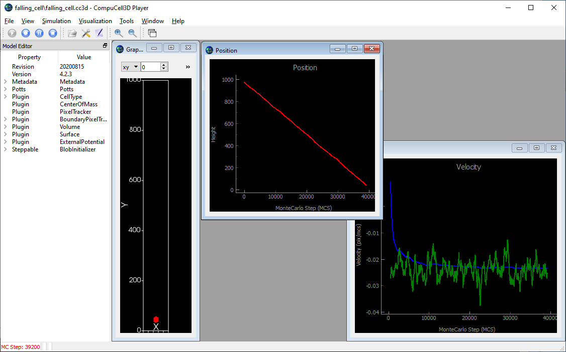
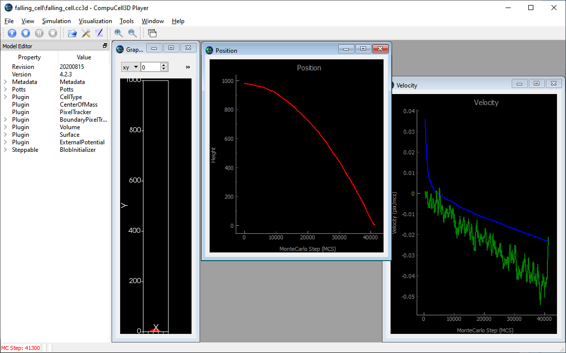
This simulation produces two graphs. One plots the cell’s Y position versus time. The second plots both the overall average (blue) and recent average (last 500 mcs, red) cell velocity.
Below is a CC3D screen shot of the “constant” case. Notice that the cell’s position versus time curve is a straight line (red line) and the velocity plots, after some large variations at the start of the simulation, settles down to a noisy constant value (blue and green lines).
Below is a CC3D screen shot of the “accelerate” case. Notice that the cell’s position versus time is a curved line (red line) and the velocity plots, after some large variations at the start of the simulation, settles down to a noisy but linearly decreasing value (blue and green lines). A linear velocity graph indicates a constant acceleration. (Note the cell’s Y coordinate is decreasing so the velocity is negative.)
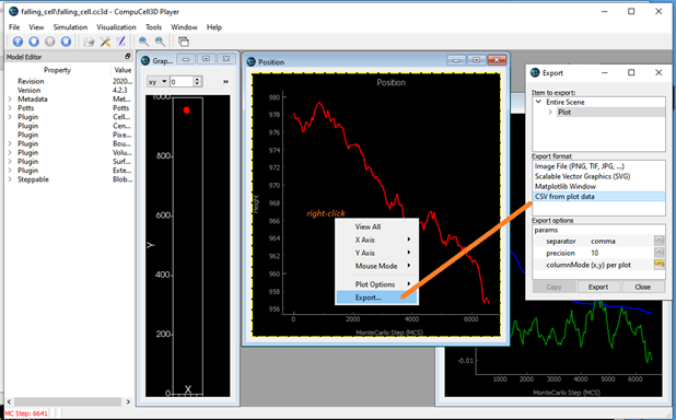
CC3D can easily export the data in a plot so you can analyze with some other program. As shown below, if you right-click in a graph window you can export the data with the “Export …” option, then select the “CSV from plot data” export format and then click the “Export” button.
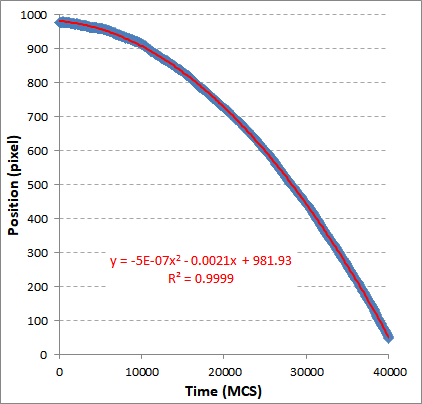
Below is the exported CC3D graph data reanalyzed in Excel. The position versus time data for the acceleration simulation is fitted with a quadratic regression line. The quadratic fit shows that the behavior is correct and the cell is accelerating.
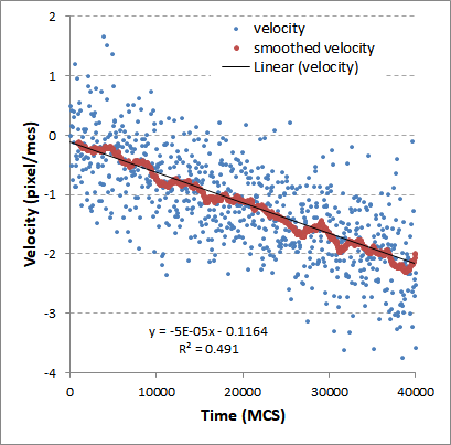
(click either graph for a larger version)
The right hand graph above is the instantaneous and smoothed velocities form the data in the left hand graph. The linear regression line’s slope is the acceleration; -5x10-5 pixel/mcs2. The behavior of the falling cell will be affected by many of the parameters in the simulation. The cell’s lambda volume and lambda surface (this simulation doesn’t use a surface constraint), the cell’s motility (aka “Potts Temperature”) and the cell’s adhesion behavior (this simulation has no adhesions) will all affect the cell’s fall rate.
Sept. 2020, J. Sluka
 CompuCell3D (Dev)

